Identifying harmful mutations in microbial populations with Tn-seq
This repository contains lesson materials, instructions, and scripts for analyzing Tn-seq data as presented during the Bodega Bay 2016 bioinformatics course.
DISCLAIMER: This lesson is written for the particular flavor of Tn-seq data generation and analysis that I am familiar with in my lab as described here, but modifications to the general Tn-seq scheme exist. Also, keep in mind that, as was determined at #ngs2015

Set up Amazon instance and install dependencies
Before we get going with data analysis, we need to set up our environment and install some dependencies. On Amazon Web Services, launch Ubuntu 14.04 LTS (64-bit) on an m3.2xlarge instance. Before you click 'Review and Launch', increase the root file system size to 30 GB. You will need to create a new private key if you do not already have one.
When the instance becomes available, copy its address, open a Terminal and connect to it via ssh:
ssh -i keyfile.pem ubuntu@copy.address.here.amazonaws.com
Now let's install software:
sudo apt-get update && sudo apt-get -y upgrade && sudo apt-get -y install autoconf automake bison build-essential default-jdk default-jre expat fastqc fastx-toolkit g++ gcc git libboost-all-dev libbz2-dev libncurses5-dev libpcre++-dev libpcre3-dev make parallel python-dev python-setuptools trimmomatic unzip wget zlib1g-dev
While I introduce my research and give an overview of Tn-seq, download and unzip the data file we'll be using:
mkdir ~/data
sudo mkfs.ext4 -E nodiscard /dev/xvdc
sudo mount /dev/xvdc ~/data
sudo chown ubuntu ~/data
cd ~/data
wget http://dib-training.ucdavis.edu.s3.amazonaws.com/2016-bodega/tnseq_reads.fastq.gz
gunzip tnseq_reads.fastq.gz && md5sum tnseq_reads.fastq.gz
This lesson is a bit of a disk hog, so let's mount the other SSD included with the m3.2xlarge instance to an analysis directory:
sudo umount /dev/xvdb
mkdir ~/analysis
sudo mount /dev/xvdb ~/analysis
sudo chown ubuntu ~/analysis
We will be using some other software packages that require manual installation. First, we'll install Heng Li's bioawk, an extension of the powerful GNU awk language which readily parses and manipulates common bioinformatics file formats like fastx and sam:
sudo mkdir /sw
sudo chown ubuntu /sw
chmod 775 /sw
cd /sw
git clone https://github.com/lh3/bioawk.git
cd bioawk
make
Next, install pullseq. I've found it to be a really handy tool for grabbing reads from fastx files by name or by matching a regular expression:
cd /sw
git clone https://github.com/bcthomas/pullseq.git
cd pullseq
./bootstrap
./configure
make
sudo make install
Install Trimmomatic:
cd /sw && wget http://www.usadellab.org/cms/uploads/supplementary/Trimmomatic/Trimmomatic-0.35.zip
unzip Trimmomatic-0.35.zip
echo 'trimmomatic=/sw/Trimmomatic-0.35/trimmomatic-0.35.jar' >> ~/.bashrc
Now let's install samtools version 1.2:
cd /sw
wget https://github.com/samtools/samtools/releases/download/1.2/samtools-1.2.tar.bz2
tar -xvjf samtools-1.2.tar.bz2
cd samtools-1.2
make
Install bowtie:
cd /sw
wget https://sourceforge.net/projects/bowtie-bio/files/bowtie/1.1.2/bowtie-1.1.2-src.zip
unzip bowtie-1.1.2-src.zip
cd bowtie-1.1.2
make
Make sure bash knows where we've installed our packages:
echo 'PATH=~/tnseq/scripts:$PATH' >> ~/.bashrc
echo 'PATH=/sw/bioawk:$PATH' >> ~/.bashrc
echo 'PATH=/sw/samtools-1.2:$PATH' >> ~/.bashrc
echo 'PATH=/sw/bowtie-1.1.2:$PATH' >> ~/.bashrc
source ~/.bashrc
which bioawk
We also need to install BioPython:
sudo easy_install pip setuptools
sudo pip install --upgrade pip setuptools
sudo -H pip install pyopenssl ndg-httpsclient pyasn1
sudo -H pip install biopython
Finally, clone the lesson repo into your home directory:
cd ~
git clone https://github.com/jbadomics/tnseq.git
Introduction to Tn-seq
In this lesson, we'll be analyzing Tn-seq data from an environmental bacterium that we study in the Bond Lab, Geobacter sulfurreducens. This organism is a model system for microbial metal reduction and extracellular electron transfer, since it obtains metabolic energy by respiring insoluble metal oxides like Fe and Mn located outside the cell. Our lab is interested in identifying the proteins involved in this remarkable ability to transfer electrons across two insulating biological membranes.
Tn-seq is a hypothesis-generating tool for identifying genes that provide fitness benefit under particular conditions. The procedure requires the following:
- A genetically tractable model organism, and
- its genome sequence.
First, cells are randomly mutagenized with a suicide plasmid containing the Mariner transposon (which confers resistance to kanamycin). This transposon is flanked by inverted repeats and integrates into the chromosome at TA sites. A saturated mutant library is created by pooling a number of colonies roughly 10 times the number of genes in the genome. This number depends on two factors:
- genome size
- GC content (higher GC microbes inherently have fewer TA sites)
The transposon mutant library we'll be looking at contains ~40,000 individual mutants. Some of them will have no phenotype; others will be lethal (i.e. the transposon insertion has interrupted an essential gene); or, the insertion will cause a fitness defect only under certain conditions.
The entire mutant library is then subjected to two or more different outgrowth conditions, ideally for a known number of cell doublings (more on this later!). Assume a mutation at locus X, which causes a fitness defect under condition 1 but not condition 2. Over a few doubling events under condition 1, cells which carry the locus X mutation will be outcompeted and eventually die off; over the same period under condition 2, cells can continue to grow despite the locus X mutation. After outgrowth, genomic DNA is harvested and submitted for Illumina sequencing to locate the genomic position where the transposon inserted. In condition 1, very few (if any reads) will map, since the mutation caused a fitness defect, whereas in condition 2, more reads will map. Genes with the highest ratios of reads mapped can then be deleted and the phenotype can be verified.
Getting down to base-ics
Let's look at the molecular steps again. 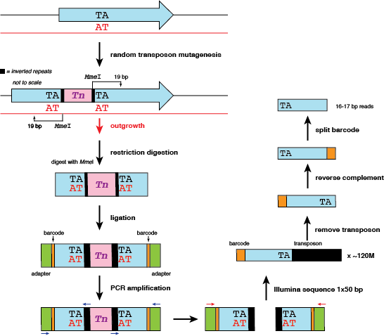
The original TA site in the genome is duplicated during the transposition event. In addition, a single transposition event will result (theoretically) in two reads that should map to the same insertion site - one on the forward strand, and one on the reverse strand. We will count this as two hits at one site.
But there's a problem: when it comes time to map reads, any read mapping to the reverse strand will need to have its insertion position corrected. Consider the following example of two mock reads mapped to the first TA site in the genome. Here is the resulting SAM file:
@HD VN:1.0  SO:unsorted
@SQ SN:chr1 LN:3820884
@PG ID:bowtie2  PN:bowtie2  VN:2.2.6    CL:"bowtie2-align-s --wrapper basic-0 -x MN1 -S test.sam -q -U simulated.fastq"
fwd_read    0   chr1    29  42  20M *   0   0   TATGGAAGAAGTTTGGCTCC    DFEEEEIDDDDDDDDDDDDD
rev_read    16  chr1    11  42  20M *   0   0   TCCCGAGAAGGTCTGGTTTA    DDDDDDDDDDDDDIEEEEFD
In column 4, we can see that the reverse read reports an alignment beginning at base 11, when in fact the TA site of insertion is at the end of the read. For this lesson, I define the coordinate of the TA site as the coordinate of the 'A' residue, which in this case is 30. We'll incorporate a step in our workflow to ensure that the forward and reverse reads arising from the same insertion event end up with an identical insertion coordinate reported.
Tn-seq data analysis workflow
Remove phiX reads
In situations where Illumina reads are generated from the same DNA template (e.g. conserved regions of the 16S rRNA gene), it can be hard to differentiate clusters on the Illumina flow cell unless an external control is spiked into the sample, usually phage phiX DNA. Your sequencing provider may say they've removed phiX reads, but let's check just to be safe.
First, create a data analysis directory:
cd ~/analysis
We'll use bowtie to map our Tn-seq reads and discard STDOUT since we're really only interested in the unmapped reads (specified with --un):
bowtie-build ~/tnseq/reference/phiX.fasta phiX
bowtie -q -p $(nproc --all) --un phiX_removed.fastq phiX ~/data/tnseq_reads.fastq > /dev/null
In this lesson I included a shell script called countseq which runs bioawk to correctly count the number of sequences in any fastq or fasta file. Make sure that phiX_removed.fastq contains fewer reads than our raw data:
countseq *.fastq
Remove transposon sequence, filter, and demultiplex
Use less to have a look at the phiX-removed reads. You should see some patterns: are there multiple barcodes? Do you see any TA insertion sites? Do the 3' ends of the reads look similar?
Previous implementations of this workflow used fastx_clipper, part of the fastx toolkit, to remove transposon sequence at the 3' end of the read. Unfortunately this was painfully slow.
Trimmomatic can do what we want, and is WAY faster. Rather than trim off Illumina adaptors, we can specify a custom file with our transposon sequence to trim:
java -Xmx28g -jar $trimmomatic SE -phred33 phiX_removed.fastq tn_removed.fastq ILLUMINACLIP:/home/ubuntu/tnseq/reference/tnseq_adapters.fa:3:30:10 MINLEN:16
Time to introduce the power of bioawk. I'm a huge fan of bioawk. We can use awk-like language to construct if statements, match regex patterns, and print reads meeting our criteria in either fasta or fastq format. In addition, bioawk automatically recognizes and parses these file formats (along with others like GFF and SAM) and assigns logical variables like $seq to describe the sequence and $qual to define the quality string.
Now we need to discard any reads that did not contain transposon sequence. By this point in our workflow, these reads can be distinguished as still being full-length (51 bp). Since we'll filter reads by length in a second, any transposon-less reads will get discarded anyway. But for possible diagnostic purposes, pull the transposon-less reads into a separate fastq file:
bioawk -c fastx '{ if(length($seq) == 51) { print "@"$name; print $seq; print "+"; print $qual; }}' tn_removed.fastq > no_transposon.fastq
Let's use bioawk again in a one-liner to capture a length distribution of the filtered reads:
bioawk -c fastx '{ print length($seq) }' tn_removed.filtered.fastq | sort | uniq -c
As we expect, the overwhelming majority of our data is 20 or 21 bp. Keep in mind that the reads still contain barcode, which we'll remove shortly. But before we get to that, run bioawk to collect the reads of desired length:
bioawk -c fastx '{ if(length($seq) >= 19 && length($seq) < 23) { print "@"$name; print $seq; print "+"; print $qual; }}' tn_removed.fastq > tn_removed.filtered.fastq
Rerun countseq to keep an eye on how many sequences we're discarding at each step:
countseq tn_removed*.fastq
When we go to map reads against the reference genome, it is critical to keep track of the genomic position where the insertion occurred. Conceptually it makes sense to reverse complement the reads so that the TA insertion sequence occurs at the 5' end:
fastx_reverse_complement -i tn_removed.filtered.fastq -o tn_removed.filtered.rc.fastq
What if a read doesn't begin with TA? This can happen sometimes, since the transposon does integrate at non-TA sites at ~2% frequency. We can safely remove the non-TA insertion reads with--you guessed it--bioawk:
bioawk -c fastx '{ if ($seq ~ /^TA/) { print "@"$name; print $seq; print "+"; print $qual; }}' tn_removed.filtered.rc.fastq > tn_removed.filtered.rc.TAonly.fastq
Just to be safe, let's write the reads that don't begin with TA to another file:
bioawk -c fastx '{ if ($seq !~ /^TA/) { print "@"$name; print $seq; print "+"; print $qual; }}' tn_removed.filtered.rc.fastq > nonTA.fastq
Take another peek at the reads with less: they should now all begin with TA and the barcode should now appear at the 3' end.
Time to separate reads by barcode. This dataset uses 3 barcodes:
BC1 CAGT parent
BC2 GACT high potential electrode outgrowth
BC3 GTGT low potential electrode outgrowth
Note that some reads end with N but should be considered as having the barcode. Bioawk can also take a regular expression:
bioawk -c fastx '{ if ($seq ~ /CAG[TN]$/) { print "@"$name; print $seq; print "+"; print $qual; }}' tn_removed.filtered.rc.TAonly.fastq > BC1.fastq
Change the regex pattern and run the same command for BC2:
bioawk -c fastx '{ if ($seq ~ /GAC[TN]$/) { print "@"$name; print $seq; print "+"; print $qual; }}' tn_removed.filtered.rc.TAonly.fastq > BC2.fastq
And for BC3:
bioawk -c fastx '{ if ($seq ~ /GTG[TN]$/) { print "@"$name; print $seq; print "+"; print $qual; }}' tn_removed.filtered.rc.TAonly.fastq> BC3.fastq
Make sure everything adds up:
countseq tn_removed*.fastq
Now, use a for loop to remove the barcode from each dataset:
for j in {1..3}; do fastx_trimmer -t 4 -i BC${j}.fastq -o BC${j}_barcode_removed.fastq; done
Map reads and collect hit statistics
Thinking ahead: when it comes time to tabulate the insertion coordinates by locus tag, the reference genome name and sequence need to match what we use to map reads to. Unfortunately this isn't always the case. The safest bet is to pull the genome sequence from the same Genbank file we'll use later for tabulating insertions. Run this little python script:
ln -s ~/tnseq/reference/Geobacter_sulfurreducens_MN1.gbk
gbk_to_fasta.py Geobacter_sulfurreducens_MN1.gbk
Now the fun can begin! Use bowtie to map reads:
bowtie-build Geobacter_sulfurreducens_MN1.fasta MN1
for j in {1..3}; do bowtie -q -p $(nproc --all) -S -n 0 -e 70 -l 28 --nomaqround -y -k 1 -a -m 1 --best --un BC${j}_unmapped.fastq MN1 BC${j}_barcode_removed.fastq BC${j}.sam; done
Take a peek at the output sam files:
less -S BC1.sam
and look at a read that mapped to the reverse strand (look for bitwise flag 16). You'll notice that the read ends in TA, which it should if it mapped to the reverse strand, but the coordinate in column 4 refers to the first base aligned reading from left to right. This means we'll need to correct the coordinate for reads mapped to the minus strand so that they have the same coordinate (i.e. TA insertion site) as the forward read that arose from the same insertion event.
How's this for a one-liner:
for j in {1..3}; do bioawk -c sam '{ if($flag==0) print $qname,$rname,$flag,$pos,$pos+1,length($seq); if($flag==16) print $qname,$rname,$flag,$pos,$pos+length($seq)-1,length($seq) }' BC${j}.sam | cut -f2,5 | sort -g -k2 | uniq -c | sed 's/^ *//' | awk -v OFS='\t' '{ print $2,$3,$1}' > BC${j}.hits.txt; done
Now have a look at BC1.hits.txt. It should be a tab-delimited text file with three columns:
- the reference sequence ID (essential for multi-contig genomes)
- the position along that reference
- the total number of transposon insertions or "hits" at that position
Collect hit statistics by gene
I am not a Python expert, but in this repo there are two scripts we'll use for converting our .hits.txt data by locus tag, using a Genbank file of the reference genome containing the annotation and coordinates of each gene feature.
mkdir tabulate && cd tabulate
tabulate_insertions.py ~/tnseq/reference/Geobacter_sulfurreducens_MN1.gbk ../BC1.hits.txt BC1 0 0.05
The last two numbers specify a percentage to trim off the N- and C-terminus, respectively, of the coding sequence. In past analyses we only consider hits within the first 95% of the total gene length
As the script runs, you'll see a scrolling output of genes that do not contain any TA site hits. What is significant about these genes?
Calculate log2 ratios to identify genes of interest
Two particular loci should jump out at us: GSU0274 and GSU3259. These genes encode inner membrane cytochromes that function at low and high potential, respectively. So, in the BC2 library (low potential electrode outgrowth), we should see very few hits in GSU0274. Likewise, in the BC3 library, we should see very few hits in GSU3259. Let's use the second script for this:
insertion_statistics_by_locustag.py /tnseq/reference/Geobacter_sulfurreducens_MN1.gbk ../BC2.hits.txt GSU0274 0 0.05
insertion_statistics_by_locustag.py /tnseq/reference/Geobacter_sulfurreducens_MN1.gbk ../BC3.hits.txt GSU3259 0 0.05